Login or Register for free to create your own customized page of blog posts from your favorite blogs. You can also add blogs by clicking the "Add to MyJacketFlap" links next to the blog name in each post.
Blog Posts by Tag
In the past 7 days
Blog Posts by Date
Click days in this calendar to see posts by day or month
Viewing: Blog Posts Tagged with: Physics &, Most Recent at Top [Help]
Results 51 - 75 of 116
How to use this Page
You are viewing the most recent posts tagged with the words: Physics & in the JacketFlap blog reader. What is a tag? Think of a tag as a keyword or category label. Tags can both help you find posts on JacketFlap.com as well as provide an easy way for you to "remember" and classify posts for later recall. Try adding a tag yourself by clicking "Add a tag" below a post's header. Scroll down through the list of Recent Posts in the left column and click on a post title that sounds interesting. You can view all posts from a specific blog by clicking the Blog name in the right column, or you can click a 'More Posts from this Blog' link in any individual post.
Fin de siècle Hungary was a progressive country. It had limited sovereignty as part of the Austro-Hungarian dual monarchy, but industry, trade, education, and social legislation were rapidly catching up with the Western World. The emancipation of Jews freed tremendous energies and opened the way for ambitious young people to the professions in law, health care, science, and engineering (though not politics, the military, and the judiciary). Excellent secular high schools appeared challenging the already established excellent denominational high schools.
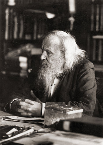
The periodic table has experienced many revisions over time as new elements have been discovered and the methods of organizing them have been solidified. Sometimes when scientists tried to fill in gaps where missing elements were predicted to reside in the periodic table, or when they made even the smallest of errors in their experiments, they came up with discoveries—often fabricated or misconstrued—that are so bizarre they could have never actually found a home in our current version of the periodic table.
Renowned English cosmologist Stephen Hawking has made his name through his work in theoretical physics as a bestselling author. His life – his pioneering research, his troubled relationship with his wife, and the challenges imposed by his disability – is the subject of a poignant biopic, The Theory of Everything. Directed by James Marsh, the film stars Eddie Redmayne, who has garnered widespread critical acclaim for his moving portrayal.
A couple of days after seeing Christopher Nolan’s Interstellar, I bumped into Sir Roger Penrose. If you haven’t seen the movie and don’t want spoilers, I’m sorry but you’d better stop reading now.
Still with me? Excellent.
Some of you may know that Sir Roger developed much of modern black hole theory with his collaborator, Stephen Hawking, and at the heart of Interstellar lies a very unusual black hole. Straightaway, I asked Sir Roger if he’d seen the film. What’s unusual about Gargantua, the black hole in Interstellar, is that it’s scientifically accurate, computer-modeled using Einstein’s field equations from General Relativity.
Scientists reckon they spend far too much time applying for funding and far too little thinking about their research as a consequence. And, generally, scientific budgets are dwarfed by those of Hollywood movies. To give you an idea, Alfonso Cuarón actually told me he briefly considered filming Gravity in space, and that was what’s officially classed as an “independent” movie. For big-budget studio blockbuster Interstellar, Kip Thorne, scientific advisor to Nolan and Caltech’s “Feynman Professor of Theoretical Physics”, seized his opportunity, making use of Nolan’s millions to see what a real black hole actually looks like. He wasn’t disappointed and neither was the director who decided to use the real thing in his movie without tweaks.
Black holes are so called because their gravitational fields are so strong that not even light can escape them. Originally, we thought these would be dark areas of the sky, blacker than space itself, meaning future starship captains might fall into them unawares. Nowadays we know the opposite is true – gravitational forces acting on the material spiralling into the black hole heat it to such high temperatures that it shines super-bright, forming a glowing “accretion disk”.
“Sir Roger Penrose.” Photo by Igor Krivokon. CC by 2.0 via Flickr.
The computer program the visual effects team created revealed a curious rainbowed halo surrounding Gargantua’s accretion disk. At first they and Thorne presumed it was a glitch, but careful analysis revealed it was behavior buried in Einstein’s equations all along – the result of gravitational lensing. The movie had discovered a new scientific phenomenon and at least two academic papers will result: one aimed at the computer graphics community and the other for astrophysicists.
I knew Sir Roger would want to see the movie because there’s a long scene where you, the viewer, fly over the accretion disk–not something made up to look good for the IMAX audience (you have to see this in full IMAX) but our very best prediction of what a real black hole should look like. I was blown away.
Some parts of the movie are a little cringeworthy, not least the oft-repeated line, “that’s relativity”. But there’s a reason for the characters spelling this out. As well as accurately modeling the black hole, the plot requires relativistic “time dilation”. Even though every physicist has known how to travel in time for over a century (go very fast or enter a very strong gravitational field) the general public don’t seem to have cottoned on.
Most people don’t understand relativity, but they’re not alone. As a science editor, I’m privileged to meet many of the world’s most brilliant people. Early in my publishing career I was befriended by Subramanian Chandrasekhar, after whom the Chandra space telescope is now named. Penrose and Hawking built on Chandra’s groundbreaking work for which he received the Nobel Prize; his The Mathematical Theory of Black Holes (1954) is still in print and going strong.
When visiting Oxford from Chicago in the 1990s, Chandra and his wife Lalitha would come to my apartment for tea and we’d talk physics and cosmology. In one of my favorite memories he leant across the table and said, “Keith – Einstein never actually understood relativity”. Quite a bold statement and remarkably, one that Chandra’s own brilliance could end up rebutting.
Space is big – mind-bogglingly so once you start to think about it, but we only know how big because of Chandra. When a giant sun ends its life, it goes supernova – an explosion so bright it outshines all the billions of stars in its home galaxy combined. Chandra deduced that certain supernovae (called “type 1a”) will blaze with near identical brightness. Comparing the actual brightness with however bright it appears through our telescopes tells us how far away it is. Measuring distances is one of the hardest things in astronomy, but Chandra gave us an ingenious yardstick for the Universe.
“Stephen Hawking.” Photo by Lwp Kommunikáció. CC by 2.0 via Flickr.
In 1998, astrophysicists were observing type 1a supernovae that were a very long way away. Everyone’s heard of the Big Bang, the moment of creation of the Universe; even today, more than 13 billion years later, galaxies continue to rush apart from each other. The purpose of this experiment was to determine how much this rate of expansion was slowing down, due to gravity pulling the Universe back together. It turns out that the expansion’s speeding up. The results stunned the scientific world, led to Nobel Prizes, and gave us an anti-gravitational “force” christened “dark energy”. It also proved Einstein right (sort of) and, perhaps for the only time in his life, Chandra wrong.
Why Chandra told me Einstein was wrong was because of something Einstein himself called his “greatest mistake”. When relativity was first conceived, it was before Edwin Hubble (after whom another space telescope is named) had discovered space itself was expanding. Seeing that the stable solution of his equations would inevitably mean the collapse of everything in the Universe into some “big crunch”, Einstein devised the “cosmological constant” to prevent this from happening – an anti-gravitational force to maintain the presumed status quo.
Once Hubble released his findings, Einstein felt he’d made a dreadful error, as did most astrophysicists. However, the discovery of dark energy has changed all that and Einstein’s greatest mistake could yet prove an accidental triumph.
Of course Chandra knew Einstein understood relativity better than almost anyone on the planet, but it frustrates me that many people have such little grasp of this most beautiful and brilliant temple of science. Well done Christopher Nolan for trying to put that right.
Interstellar is an ambitious movie – I’d call it “Nolan’s 2001” – and it educates as well as entertains. While Matthew McConaughey barely ages in the movie, his young daughter lives to a ripe old age, all based on what we know to be true. Some reviewers have criticized the ending – something I thought I wouldn’t spoil for Sir Roger. Can you get useful information back out of a black hole? Hawking has changed his mind, now believing such a thing is possible, whereas Penrose remains convinced it cannot be done.
We don’t have all the answers, but whichever one of these giants of the field is right, Nolan has produced a thought-provoking and visually spectacular film.
Image Credit: “Best-Ever Snapshot of a Black Hole’s Jets.” Photo by NASA Goddard Space Flight Center. CC by 2.0 via Flickr.
Many attempts have been made to explain the historic and current lack of women working in STEM fields. During her two years of service as Director of Policy Planning for the US State Department, from 2009 to 2011, Anne-Marie Slaughter suggested a range of strategies for corporate and political environments to better support women at work. These spanned from social-psychological interventions to the introduction of role models and self-affirmation practices. Slaughter has written and spoken extensively on the topic of equality between men and women. Beyond abstract policy change, and continuing our celebration of women in STEM, there are practical tips and guidance for young women pursuing a career in Science, Technology, Engineering, or Mathematics.
(1) &nsbp; Be open to discussing your research with interested people.
From in-depth discussions at conferences in your field to a quick catch up with a passing colleague, it can be endlessly beneficial to bounce your ideas off a range of people. New insights can help you to better understand your own ideas.
(2) &nsbp; Explore research problems outside of your own.
Looking at problems from multiple viewpoints can add huge value to your original work. Explore peripheral work, look into the work of your colleagues, and read about the achievements of people whose work has influenced your own. New information has never been so discoverable and accessible as it is today. So, go forth and hunt!
Meeting by StartupStockPhotos. Public domain via Pixabay.
(3) &nsbp; Collaborate with people from different backgrounds.
The chance of two people having read exactly the same works in their lifetime is nominal, so teaming up with others is guaranteed to bring you new ideas and perspectives you might never have found alone.
(4) &nsbp; Make sure your research is fun and fulfilling.
As with any line of work, if it stops being enjoyable, your performance can be at risk. Even highly self-motivated people have off days, so look for new ways to motivate yourself and drive your work forward. Sometimes this means taking some time to investigate a new perspective or angle from which to look at what you are doing. Sometimes this means allowing yourself time and distance from your work, so you can return with a fresh eye and a fresh mind!
(5) &nsbp; Surround yourself with friends who understand your passion for scientific research.
The life of a researcher can be lonely, particularly if you are working in a niche or emerging field. Choose your company wisely, ensuring your valuable time is spent with friends and family who support and respect your work.
Image Credit: “Board” by blickpixel. Public domain via Pixabay.
Galileo and some of his contemporaries left careful records of their telescopic observations of sunspots – dark patches on the surface of the sun, the largest of which can be larger than the whole earth. Then in 1844 a German apothecary reported the unexpected discovery that the number of sunspots seen on the sun waxes and wanes with a period of about 11 years.
Initially nobody considered sunspots as anything more than an odd curiosity. However, by the end of the nineteenth century, scientists started gathering more and more data that sunspots affect us in strange ways that seemed to defy all known laws of physics. In 1859 Richard Carrington, while watching a sunspot, accidentally saw a powerful explosion above it, which was followed a few hours later by a geomagnetic storm – a sudden change in the earth’s magnetic field. Such explosions – known as solar flares – occur more often around the peak of the sunspot cycle when there are many sunspots. One of the benign effects of a large flare is the beautiful aurora seen around the earth’s poles. However, flares can have other disastrous consequences. A large flare in 1989 caused a major electrical blackout in Quebec affecting six million people.
Interestingly, Carrington’s flare of 1859, the first flare observed by any human being, has remained the most powerful flare so far observed by anybody. It is estimated that this flare was three times as powerful as the 1989 flare that caused the Quebec blackout. The world was technologically a much less developed place in 1859. If a flare of the same strength as Carrington’s 1859 flare unleashes its full fury on the earth today, it will simply cause havoc – disrupting electrical networks, radio transmission, high-altitude air flights and satellites, various communication channels – with damages running into many billions of dollars.
There are two natural cycles – the day-night cycle and the cycle of seasons – around which many human activities are organized. As our society becomes technologically more advanced, the 11-year cycle of sunspots is emerging as the third most important cycle affecting our lives, although we have been aware of its existence for less than two centuries. We have more solar disturbances when this cycle is at its peak. For about a century after its discovery, the 11-year sunspot cycle was a complete mystery to scientists. Nobody had any clue as to why the sun has spots and why spots have this cycle of 11 years.
A first breakthrough came in 1908 when Hale found that sunspots are regions of strong magnetic field – about 5000 times stronger than the magnetic field around the earth’s magnetic poles. Incidentally, this was the first discovery of a magnetic field in an astronomical object and was eventually to revolutionize astronomy, with subsequent discoveries that nearly all astronomical objects have magnetic fields. Hale’s discovery also made it clear that the 11-year sunspot cycle is the sun’s magnetic cycle.
Sunspot 1-20-11, by Jason Major. CC BY-NC-SA 2.0 via Flickr.
Matter inside the sun exists in the plasma state – often called the fourth state of matter – in which electrons break out of atoms. Major developments in plasma physics within the last few decades at last enabled us to systematically address the questions of why sunspots exist and what causes their 11-year cycle. In 1955 Eugene Parker theoretically proposed a plasma process known as the dynamo process capable of generating magnetic fields within astronomical objects. Parker also came up with the first theoretical model of the 11-year cycle. It is only within the last 10 years or so that it has been possible to build sufficiently realistic and detailed theoretical dynamo models of the 11-year sunspot cycle.
Until about half a century ago, scientists believed that our solar system basically consisted of empty space around the sun through which planets were moving. The sun is surrounded by a million-degree hot corona – much hotter than the sun’s surface with a temperature of ‘only’ about 6000 K. Eugene Parker, in another of his seminal papers in 1958, showed that this corona will drive a wind of hot plasma from the sun – the solar wind – to blow through the entire solar system. Since the earth is immersed in this solar wind – and not surrounded by empty space as suspected earlier – the sun can affect the earth in complicated ways. Magnetic fields created by the dynamo process inside the sun can float up above the sun’s surface, producing beautiful magnetic arcades. By applying the basic principles of plasma physics, scientists have figured out that violent explosions can occur within these arcades, hurling huge chunks of plasma from the sun that can be carried to the earth by the solar wind.
The 11-year sunspot cycle is only approximately cyclic. Some cycles are stronger and some are weaker. Some are slightly longer than 11 years and some are shorter. During the seventeenth century, several sunspot cycles went missing and sunspots were not seen for about 70 years. There is evidence that Europe went through an unusually cold spell during this epoch. Was this a coincidence or did the missing sunspots have something to do with the cold climate? There is increasing evidence that sunspots affect the earth’s climate, though we do not yet understand how this happens.
Can we predict the strength of a sunspot cycle before its onset? The sunspot minimum around 2006–2009 was the first sunspot minimum when sufficiently sophisticated theoretical dynamo models of the sunspot cycle existed and whether these models could predict the upcoming cycle correctly became a challenge for these young theoretical models. We are now at the peak of the present sunspot cycle and its strength agrees remarkably with what my students and I predicted in 2007 from our dynamo model. This is the first such successful prediction from a theoretical model in the history of our subject. But is it merely a lucky accident that our prediction has been successful this time? If our methodology is used to predict more sunspot cycles in the future, will this success be repeated?
Headline image credit: A spectacular coronal mass ejection, by Steve Jurvetson. CC-BY-2.0 via Flickr.
It is becoming widely accepted that women have, historically, been underrepresented and often completely written out of work in the fields of Science, Technology, Engineering, and Mathematics (STEM). Explanations for the gender gap in STEM fields range from genetically-determined interests, structural and territorial segregation, discrimination, and historic stereotypes. As well as encouraging steps toward positive change, we would also like to retrospectively honour those women whose past works have been overlooked.
From astronomer Caroline Herschel to the first female winner of the Fields Medal, Maryam Mirzakhani, you can use our interactive timeline to learn more about the women whose works in STEM fields have changed our world.
With free Oxford University Press content, we tell the stories and share the research of both famous and forgotten women.
Featured image credit: Microscope. Public Domain via Pixabay.
Modern science has introduced us to many strange ideas on the universe, but one of the strangest is the ultimate fate of massive stars in the Universe that reached the end of their life cycles. Having exhausted the fuel that sustained it for millions of years of shining life in the skies, the star is no longer able to hold itself up under its own weight, and it then shrinks and collapses catastrophically unders its own gravity. Modest stars like the Sun also collapse at the end of their life, but they stabilize at a smaller size. But if a star is massive enough, with tens of times the mass of the Sun, its gravity overwhelms all the forces in nature that might possibly halt the collapse. From a size of millions of kilometers across, the star then crumples to a pinprick size, smaller than even the dot on an “i”.
What would be the final fate of such massive collapsing stars? This is one of the most exciting questions in astrophysics and modern cosmology today. An amazing inter-play of the key forces of nature takes place here, including gravity and quantum forces. This phenomenon may hold the secrets to man’s search for a unified understanding of all forces of nature, with exciting implications for astronomy and high energy astrophysics. Surely, this is an outstanding unresolved mystery that excites physicists and the lay person alike.
The story of massive collapsing stars began some eight decades ago when Subrahmanyan Chandrasekhar probed the question of final fate of stars such as the Sun. He showed that such a star, on exhausting its internal nuclear fuel, would stabilize as a “White Dwarf”, about a thousand kilometers in size. Eminent scientists of the time, in particular Arthur Eddington, refused to accept this, saying how a star can ever become so small. Finally Chandrasekhar left Cambridge to settle in the United States. After many years, the prediction was verified. Later, it also became known that stars which are three to five times the Sun’s mass give rise to what are called Neutron stars, just about ten kilometers in size, after causing a supernova explosion.
But when the star has a mass more than these limits, the force of gravity is supreme and overwhelming. It overtakes all other forces that could resist the implosion, to shrink the star in a continual gravitational collapse. No stable configuration is then possible, and the star which lived millions of years would then catastrophically collapse within seconds. The outcome of this collapse, as predicted by Einstein’s theory of general relativity, is a space-time singularity: an infinitely dense and extreme physical state of matter, ordinarily not encountered in any of our usual experiences of physical world.
Cradle of stars, photo by Scott Cresswell CC-by-2.0 via Flickr
As the star collapses, an ‘event horizon’ of gravity can possibly develop. This is essentially ‘a one way membrane’ that allows entry, but no exits permitted. If the star entered the horizon before it collapsed to singularity, the result is a ‘Black Hole’ that hides the final singularity. It is the permanent graveyard for the collapsing star.
As per our current understanding of physics, it was one such singularity, the ‘Big Bang’, that created our expanding universe we see today. Such singularities will be again produced when massive stars die and collapse. This is the amazing place at boundary of Cosmos, a region of arbitrarily large densities billions of times the Sun’s density.
An enormous creation and destruction of particles takes place in the vicinity of singularity. One could imagine this as ‘cosmic inter-play’ of basic forces of nature coming together in a unified manner. The energies and all physical quantities reach their extreme values, and quantum gravity effects dominate this regime. Thus, the collapsing star may hold secrets vital for man’s search for a unified understanding of forces of nature.
The question then arises: Are such super-ultra-dense regions of collapse visible to faraway observers, or would they always be hidden in a black hole? A visible singularity is sometimes called a ‘Naked Singularity’ or a ‘Quantum Star’. The visibility or otherwise of such super-ultra-dense fireball the star has turned into, is one of the most exciting and important questions in astrophysics and cosmology today, because when visible, the unification of fundamental forces taking place here becomes observable in principle.
A crucial point is, while gravitation theory implies that singularities must form in collapse, we have no proof the horizon must necessarily develop. Therefore, an assumption was made that an event horizon always does form, hiding all singularities of collapse. This is called ‘Cosmic Censorship’ conjecture, which is the foundation of current theory of black holes and their modern astrophysical applications. But if the horizon did not form before the singularity, we then observe the super-dense regions that form in collapsing massive stars, and the quantum gravity effects near the naked singularity would become observable.
“It turns out that the collapse of a massive star will give rise to either a black hole or naked singularity”
In recent years, a series of collapse models have been developed where it was discovered that the horizon failed to form in collapse of a massive star. The mathematical models of collapsing stars and numerical simulations show that such horizons do not always form as the star collapsed. This is an exciting scenario because the singularity being visible to external observers, they can actually see the extreme physics near such ultimate super-dense regions.
It turns out that the collapse of a massive star will give rise to either a black hole or naked singularity, depending on the internal conditions within the star, such as its densities and pressure profiles, and velocities of the collapsing shells.
When a naked singularity happens, small inhomogeneities in matter densities close to singularity could spread out and magnify enormously to create highly energetic shock waves. This, in turn, have connections to extreme high energy astrophysical phenomena, such as cosmic Gamma rays bursts, which we do not understand today.
Also, clues to constructing quantum gravity–a unified theory of forces, may emerge through observing such ultra-high density regions. In fact, the recent science fiction movie Interstellar refers to naked singularities in an exciting manner, and suggests that if they did not exist in the Universe, it would be too difficult then to construct a quantum theory of gravity, as we will have no access to experimental data on the same!
Shall we be able to see this ‘Cosmic Dance’ drama of collapsing stars in the theater of skies? Or will the ‘Black Hole’ curtain always hide and close it forever, even before the cosmic play could barely begin? Only the future observations of massive collapsing stars in the universe would tell!
A previous blog post, Patterns in Physics, discussed alternative “representations” in physics as akin to languages; an underlying quantum reality described in either a position or a momentum representation. Both are equally capable of a complete description, the underlying reality itself residing in a complex space with the very concepts of position/momentum or wave/particle only relevant in a “classical limit”. The history of physics has progressively separated such incidentals of our description from what is essential to the physics itself. We will consider this for time itself here.
Thus, consider the simple instance of the motion of a ball from being struck by a bat (A) to being caught later at a catcher’s hand (B). The specific values given for the locations of A and B or the associated time instants are immediately seen as dependent on each person in the stadium being free to choose the origin of his or her coordinate system. Even the direction of motion, whether from left to right or vice versa, is of no significance to the physics, merely dependent on which side of the stadium one is sitting.
All spectators sitting in the stands and using their own “frame of reference” will, however, agree on the distance of separation in space and time of A and B. But, after Einstein, we have come to recognize that these are themselves frame dependent. Already in Galilean and Newtonian relativity for mechanical motion, it was recognized that all frames travelling with uniform velocity, called “inertial frames”, are equivalent for physics so that besides the seated spectators, a rider in a blimp moving overhead with uniform velocity in a straight line, say along the horizontal direction of the ball, is an equally valid observer of the physics.
Einstein’s Special Theory of Relativity, in extending the equivalence of all inertial frames also to electromagnetic phenomena, recognized that the spatial separation between A and B or, even more surprisingly to classical intuition, the time interval between them are different in different inertial frames. All will agree on the basics of the motion, that ball and bat were coincident at A and ball and catcher’s hand at B. But one seated in the stands and one on the blimp will differ on the time of travel or the distance travelled.
Even on something simpler, and already in Galilean relativity, observers will differ on the shape of the trajectory of the ball between A and B, all seeing parabolas but of varying “tightness”. In particular, for an observer on the blimp travelling with the same horizontal velocity as that of the ball as seen by the seated, the parabola degenerates into a straight up and down motion, the ball moving purely vertically as the stadium itself and bat and catcher slide by underneath so that one or the other is coincident with the ball when at ground level.
Hourglass, photo by Erik Fitzpatrick, CC-BY-2.0 via Flickr
There is no “trajectory of the ball’s motion” without specifying as seen by which observer/inertial frame. There is a motion, but to say that the ball simultaneously executes many parabolic trajectories would be considered as foolishly profligate when that is simply because there are many observers. Every observer does see a trajectory, but asking for “the real trajectory”, “What did the ball really do?”, is seen as an invalid, or incomplete, question without asking “as seen by whom”. Yet what seems so obvious here is the mistake behind posing as quantum mysteries and then proposing as solutions whole worlds and multiple universes(!). What is lost sight of is the distinction between the essential physics of the underlying world and our description of it.
The same simple problem illustrates another feature, that physics works equally well in a local time-dependent or a global, time-independent description. This is already true in classical physics in what is called the Lagrangian formulation. Focusing on the essential aspects of the motion, namely the end points A and B, a single quantity called the action in which time is integrated over (later, in quantum field theory, a Lagrangian density with both space and time integrated over) is considered over all possible paths between A and B. Among all these, the classical motion is the one for which the action takes an extreme (technically, stationary) value. This stationary principle, a global statement over all space and time and paths, turns out to be exactly equivalent to the local Newtonian description from one instant to another at all times in between A and B.
There are many sophisticated aspects and advantages of the Lagrangian picture, including its natural accommodation of basic conservation laws of energy, momentum and angular momentum. But, for our purpose here, it is enough to note that such stationary formulations are possible elsewhere and throughout physics. Quantum scattering phenomena, where it seems natural to think in terms of elapsed time during the collisional process, can be described instead in a “stationary state” picture (fixed energy and standing waves), with phase shifts (of the wave function) that depend on energy, all experimental observables such as scattering cross-sections expressed in terms of them.
“The concept of time has vexed humans for centuries, whether layman, physicist or philosopher”
No explicit invocation of time is necessary although if desired so-called time delays can be calculated as derivatives of the phase shifts with respect to energy. This is because energy and time are quantum-mechanical conjugates, their product having dimensions of action, and Planck’s quantum constant with these same dimensions exists as a fundamental constant of our Universe. Indeed, had physicists encountered quantum physics first, time and energy need never have been invoked as distinct entities, one regarded as just Planck’s constant times the derivative (“gradient” in physics and mathematics parlance) of the other. Equally, position and momentum would have been regarded as Planck’s constant times the gradient in the other.
The concept of time has vexed humans for centuries, whether layman, physicist or philosopher. But, making a distinction between representations and an underlying essence suggests that space and time are not necessary for physics. Together with all the other concepts and words we perforce have to use, including particle, wave, and position, they are all from a classical limit with which we try to describe and understand what is actually a quantum world. As long as that is kept clearly in mind, many mysteries and paradoxes are dispelled, seen as artifacts of our pushing our models and language too far and “identifying” them with the underlying reality that is in principle out of reach.
In the last of the Physics Project Lab blog posts, Paul Gluck, co-author of Physics Project Lab, describes how to create and investigate the domino effect…
Many dominoes may be stacked in a row separated by a fixed distance, in all sorts of interesting formations. A slight push to the first domino in the row results in the falling of the whole stack. This is the domino effect, a term also used in figuratively in a political context.
You can use this amusing phenomenon to carry out a little project in physics. Instead of dominoes it’s preferable to use units that are uniformly smooth on both sides, say for example building blocks for kids. Chuildren’s building blocks usually come in sets of 100, 200 or 280 blocks.
The blocks are stacked in a perfect straight line, absolutely uniformly spaced. To ensure this, lay them along the extended metal strip of a builder’s ruler several meters long, fixed at both ends. A non polished wooden floor is a suitable surface, since its roughness is enough to prevent any sliding of the blocks while falling.
What is interesting to measure and correlate in your experimentation? You want to measure the speed of the pulse when the first block is given a reproducibly slight push. In other words, you must measure the total length of the stack, as well as the time between the beginning of the fall of the first block and the fall of the last one. The speed will then be the total distance divided by the time elapsed.
Domino Rally, by mikeyp2000. CC-BY-NC-2.0 via Flickr.
There are several questions you can ask and investigate. First, how does the spacing between the blocks affect the pulse speed? Second, for the same spacing, how do the pulse speeds compare between two cases: the first, with the regular blocks, and the second when you double the height of each block (by sticking two blocks on top of each other to form a single block)? Third, for large numbers of units N in the stack, does the speed depend on the number of units (say when N = 100 and when N = 200)? Finally, does the speed vary for small numbers of units in the stack, say for values between 5 and 15?
For fair comparison between the various cases, you must devise a way to give the slight initial push reproducibly. One way you can arrange this is by releasing a pendulum above the first block and releasing it from a fixed distance so that at the end of its swing the bob just touches the first block, causing it to fall.
For time measurements you need a stopwatch. Be aware that you have a reaction time between when you perceive any event and the pressing of the stopwatch – this can be anything from 0.1 to 0.3 seconds. So repeat each measurement a number of times and take the average. If you have access to two photogates in a physics lab, you can devise a more accurate way of measuring the pulse speed. Actuate the first one by the beginning of the fall of the first block, the second one by the fall of the last one. Couple the two photogates by a circuit that triggers measuring the time when the first brick starts to fall and stops measuring it when the second block falls. You can also video the whole event and analyze the clip frame-by-frame to calculate times.
Happy tinkering!
We hope you have enjoyed the Physics Project Lab series. Have you tried this experiment or any of the other experiments at home? Tell us how it went to get the chance to win a free copy of ‘Physics Project Lab’. We’ll pick our favourite descriptions on 9th January.
Although we rarely stop to think about the origin of the elements of our bodies, we are directly connected to the greater universe. In fact, we are literally made of stardust that was liberated from the interiors of dying stars in gigantic explosions, and then collected to form our Earth as the solar system took shape some 4.5 billion years ago. Until about two decades ago, however, we knew only of our own planetary system so that it was hard to know for certain how planets formed, and what the history of the matter in our bodies was.
Then, in 1995, the first planet to orbit a distant Sun-like star was discovered. In the 20 years since then, thousands of others have been found. Most planets cannot be detected with our present-day technologies, but estimates based on those that we have observed suggest that almost every star in the sky has at least one extrasolar planet (or exoplanet) orbiting it. That means that there are more than 100 billion planetary systems in our Milky Way Galaxy alone! Imagine that: astronomers have gone from knowing of 1 planetary system to some 100 billion, in the same decades in which human genome scientists sequenced the 6 billion base-pairs that lie at the foundation of our bodies. How many of these planetary systems could potentially support life, and would that life use a similar code?
Exoplanets are much too far away to be actually imaged, and they are way too faint to be directly observed next to the bright glow of the stars they orbit. Therefore, the first exoplanet discoveries were made through the gravitational tug on their central star during their orbits. This pull moves the star slightly back and forth. Only relatively heavy, close-in planets can be detected that way, using the repeating Doppler shifts of their central star’s light from red to blue and back. Another way to find planets is to measure how they block the light of their central star if they happen to cross in front of it as seen from Earth. If they are seen to do this twice or more, the temporary dimmings of their star’s light can disclose the planet’s size and distance to its star (basically using the local “year” – the time needed to orbit its star – for these calculations). If both the gravitational tug and the dimming profile can be measured, then even the mass of the planet can be estimated. Size and mass together give an average density from which, in turn, knowledge of the chemical composition of that planet comes within reach.
Star trails, by MLazarevski. CC-BY-ND-2.0 via Flickr.
With the discoveries of so many planets, we have realized that an astonishing diversity exists: hot Jupiter-sized planets that orbit closer to their star than Mercury orbits the Sun, quasi-Earth-sized planets that may have rain showers of molten iron or glass, frozen planets around faintly-glowing red dwarf stars, and possibly some billions of Earth-sized planets at distances from their host stars where liquid water could exist on the surface, possibly supporting life in a form that we might recognize if we saw it.
Guided by these recent observations, mega-computers programmed with the laws of physics give us insight into how these exo-worlds are formed, from their initial dusty disks to the eventual complement of star-orbiting planets. We can image the disks directly by focusing on the faint infrared glow of their gas and dust that is warmed by their proximity to their star. We cannot, however, directly see these far-away planets, at least not yet. But now, for the first time, we can at least see what forming planets do to the gas and dust around them in the process of becoming a mature heavenly body.
A new observatory, called ALMA, working with microwaves that lie even beyond the infrared color range, has been built in the dry Atacama desert in Chili. ALMA was pointed at a young star, hundreds of light years away. Its image of that target star, LH Tauri, not only shows the star itself and the disk around it, but also a series of dark rings that are most likely created as the newly forming planets pull in the gas and dust around them. The image is of stunning quality: it shows details down to a resolution equivalent to the width of a finger seen at a distance of 50 km (30 miles).
At the distance of LH Tauri, even that stunning imaging capability means that we can see structures only if these are larger than about the distance of the Sun out to Jupiter, so there is a long way yet to go before we see anything like the planet directly. But we will observe more of these juvenile planetary systems just past the phase of their birth. And images like that give us a glimpse of what happened in our own planetary system over 4.5 billion years ago, before the planets were fully formed, pulling in the gases and dust that we now live on, and that ultimately made their way to the cycles of our own planet, to constitute all living beings on Earth.
What a stunning revolution: from being part of the only planetary system we knew of, we have been put among billions and billions of neighbors. We remember Galileo Galilei for showing us that the Sun and not the Earth was the center of the solar system. Will our society remember the names of those who proved that billions of planets exist all over the Galaxy?
Headline image credit: Star shower, by c@rljones. CC-BY-NC-2.0 via Flickr.
Many of you have likely seen the beautiful grand spiral galaxies captured by the likes of the Hubble space telescope. Images such as those below of the Pinwheel and Whirlpool galaxies display long striking spiral arms that wind into their centres. These huge bodies represent a collection of many billions of stars rotating around the centre at hundreds of kilometers per second. Also contained within is a tremendous amount of gas and dust, not much different from that found here on Earth, seen as dark patches on the otherwise bright galactic disc.
Pinwheel and whirlpool spiral galaxies, a.k.a. M101 and M51:
Yet, rather embarrassingly, whilst we have many remarkable images of a veritable zoo of galaxies from across the Universe, we have surprisingly little knowledge of the appearance and structure of our own galaxy (the Milky Way). We do not know with certainty for example how many spiral arms there are. Does it have two, four, or no clear structure? Is there an inner bar (a long thin concentration of stars and gas), and if so does it rotate with the arms, or faster than them? Unfortunately we cannot simply take a picture from outside the galaxy as we can with those above, even if we could travel at the speed of light it would take tens of thousands of years to get far away enough to get a good picture!
The main difficulty comes from that we are located inside the disc of our galaxy. Just as we cannot know what the exterior of a building looks like if we are stuck inside it, we cannot get a good picture of what our own galaxy looks like from the Earth’s position. To build a map of our galaxy we rely on measuring the speeds of stars and gas, which we then convert to distances by making some assumptions of the structure. However the uncertainty in these distances is high, and despite a multitude of measurements we have no resounding consensus on the exact shape of our galaxy.
Movie showing how spiral arms (left) appear in velocity space (right).
There is, however, a way around this problem. Instead of trying to calculate distances, we can simply look at the speed of the observed material in the galaxy. The movie above shows the underlying concept. By measuring the speed of material along the line of sight from where the Earth is located in the galaxy, you built up a pseudo-map of the structure. In this example the grey disc is the structure you would see if the galaxy were a featureless disc. If we then superimpose some arm features, where the amount of stars and gas is greater than that in the rest of the galaxy, we see the arms clearly appear in our velocity map. Maps of this kind exist for our galaxy, with those for hydrogen and carbon monoxide (shown below) gas displaying the best arm features.
This may appear the problem is solved; we can simply trace the arm features and map them back onto a top-down map. Unfortunately doing so introduces the problems as measuring distances in the first place, and there is no single solution for mapping material from velocity to position space.
A different approach is to try and reproduce the map shown above by making informed estimates of what we believe the galaxy may look like. If we choose some top-down structure that re-creates the velocity map shown above, that we have observed directly from here on Earth, then we can assume the top-down map is also a reasonable map of the Milky Way.
Our work then began on a large number of simulations investigating the many different possibilities for the shape of the galaxy, investigating such parameters as the number of arms and speed of the bar. Care had to be taken with creating the velocity map, as what is actually measured by observations is the emission of the gas (akin to temperature). This can be absorbed and re-emitted by any additional gas the emission may pass through en route to the Earth.
In the two videos below are our best-fitting maps found for a two armed and four-armed model. Two arms tend not to produce enough structure, while the four-armed models can reproduce many of the features. Unfortunately it is very difficult to match all the features at the same time. This suggests that the arms of the galaxy may be of some irregular shape, and are not well encompassed by some regular, symmetric spiral pattern. This still leaves the question somewhat open, but also informs us that we need to investigate more irregular shapes and perhaps more complex physical processes to finally build a perfect top-down map of our galaxy.
Over the next few weeks, Paul Gluck, co-author of Physics Project Lab, will be describing how to conduct various different Physics experiments. In his third post, Paul explains how to investigate and experiment with rubber bands…
Rubber bands are unusual objects, and behave in a manner which is counterintuitive. Their properties are reflected in characteristic mechanical, thermal and acoustic phenomena. Such behavior is sufficiently unusual to warrant quantitative investigation in an experimental project.
A well-known phenomenon is the following. When you stretch a rubber band suddenly and immediately touch your lips with it, it feels warm, the rubber band gives off heat.
Unlike usual objects, which expand when heated, a rubber band contracts when you heat it. To see this, suspend a rubber band vertically and attach a weight to it. Measure carefully its stretched length by a ruler placed along it. Now blow hot air on the rubber band from a hair dryer, thus heating it. Measure the new length and ascertain that the band contracted.
The behaviour is also strange when you try to see how the length of a rubber band depends on whether you load or unload it. To see this, suspend a rubber band, affix to its bottom a cup to hold weights, as shown.
Now increase the weights in the cup in measured equal increments, and for each weight measure the length, and the change in length from the unstretched state, of the rubber band by a meter stick laid along it.
Force versus length with hysteresis, image provided by Paul Gluck
For each weight, wait two minutes before the new length measurement Record your results. Now reverse the process: unload the weights one by one, and measure the resulting lengths.
For each amount of weight, will the rubber band have the same length when loading as when unloading? No, the behavior is much more subtle and is shown in the graph, in which one path results when loading, the other when unloading. This effect is known as hysteresis, and is related to energy losses in the band.
What happens to the sound of a plucked rubber band?
Try it: pluck a rubber band while gradually stretching it, thereby increasing the tension in it. In the process the plucking produces a pitch which is practically unchanged. But if you keep the length of a rubber band constant but increase the tension in it somehow, the pitch will change. You can keep the length constant, while changing the tension, as follows: fix one end of the rubber band or strip. Pass the free end over a little pulley, affix a cup to that end to hold weights, then putting increasing amounts of weight into the cup will increase the tension in the rubber band, while keeping its length constant.
Unless you have perfect pitch and can detect small differences in pitch, you may need more sensitive means to detect the variations. One way is to have a tiny microphone nearby that will pick up the sound produced when you pluck the band. This sound is then passed on to a software (on the Web search for ‘free acoustic spectrum analyzer’) which analyzes the sounds and tells what frequencies are present in the plucking sound.
Finally, how does a flat thin rubber strip transmit light? Take a very thin flat rubber strip and start stretching it. Now shine a strong spotlight close to one side of the strip and measure the intensity of the light which is transmitted on to its other side, while the strip is stretched. You would expect that as the strip is stretched it becomes thinner so more light should get through, right? Wrong: for some region of stretching the transmitted light intensity may actually decrease.
If you have access to a physics lab and modern sensors you can set up an apparatus which will allow to explore in depth the whole range of phenomena to greater accuracy.
Have you tried this experiment at home? Tell us how it went to get the chance to win a free copy of the Physics Project Lab book! We’ll pick our favourite descriptions on 9th January.
Over the next few weeks, Paul Gluck, co-author of Physics Project Lab, will be describing how to conduct various different Physics experiments. In his second post, Paul explains how to build your own drinking bird and study its behaviour in varying ways:
You may have seen the drinking bird toy in action. It dips its beak into a full glass of water in front of it, after which it swings to and fro for a while, returns to drink some more, and so on, seemingly forever. You can buy one on the internet for a few dollars, and perform with it a fascinating physics project.
But how does it work?
A dyed volatile liquid partially fills a tube fitted with glass bulbs at both ends. The lower end of the tube dips into the liquid in the bottom bulb, the body. The upper bulb, the head, holds a beak which serves two functions. First, it shifts the center of mass forward. Secondly, when the bird is horizontal its head dips into a beaker of liquid (usually water), so that the felt covering soaks up some of the liquid. As the moisture in the felt evaporates it cools the top bulb, and some of the vapor within it condenses, thereby reducing the vapor pressure of the internal liquid below that in the bottom bulb. As a result, liquid is forced upward into the head, moving the center of mass forward. The top-heavy bird tips forward and the beak dips into the water. As the bird tips forward, the bottom end of the tube rises above the liquid surface in the bulb; vapor can bubble up from the bottom end of the tube to the top, displacing some liquid in the head, making it flow back to the bottom. The weight of the liquid in the bulb will restore the device to the vertical position, and so on, repeating the cycle of motion. The liquid within is warmed and cooled in each cycle. The cycle is maintained as long as there is water to wet the beak.
‘A drinking bird’, image provided by Paul Gluck and used with permission
The rate of evaporation from the beak depends on the temperature and humidity of the surroundings. These parameters will influence the period of the motion. Forced convection will strongly enhance the evaporation and affect the period. Such enhancement will also be created by the air flow caused by the swinging motion of the bird.
Here are some suggestions for studying the behaviour of the swinging bird, at various degrees of sophistication.
Measure the period of motion of the bird and the evaporation rate, and relate the two to each other. You can do this also when water in the beaker is replaced by another liquid, say alcohol. To measure the evaporation rate the bird may be placed on a sensitive electronic balance, accurate to 0.001 g. A few drops of the external liquid may be applied to the felt of the head by a pipette. Measure the time variation of the mass of this liquid, and that of the period of motion, without replenishing the liquid when the bird bows into its horizontal position. Allow for the time spent in the horizontal position. Establish experimentally the time range for which the evaporation may be taken as constant.
Explore how forced convection, say from a small fan directed at the head, changes the rate of evaporation, and thereby the period of the motion.
The effects of humidity on the period may be observed as follows: build a transparent plexiglass container with a small opening. Place the bird inside. Vary the internal humidity by injecting controlled amounts of fine spray into the enclosed space. You can do this by using the atomizer of a perfume bottle.
By taking a video of the motion and analyzing it frame-by-frame using a frame grabber, measure the angle of inclination of the bird to the vertical as a function of time.
Do away altogether with the beaker of liquid in front of the bird and show that all it needs for oscillatory motion is the presence of a difference of temperature between the bottom and the top, a temperature gradient. To do this, paint the lower bulb and the tube black, and shine a flood lamp on them at controlled distances, while shielding the head, so as to create a temperature gradient between head and body. Such heating increases the vapor pressure within, causing liquid to be forced up into the head and making the toy dip, just as for the cooling of the head by evaporation. It will then be interesting to study how the time elapsed before the first swing and the period of motion are related to the effective surface being illuminated (how would you measure that?), and to the effective energy supplied to the bird which itself will depend on the lamp’s distance from the bird
There are many more topics that can be investigated. As one example, you could follow the time dependence of the head and stem temperatures in each cycle by means of tiny thermocouples, correlating these with the angular motion of the bird. Heat enters the tube and is transported to the head, and this will be reflected in a steady state temperature difference between the two. Both head and tube temperatures may vary during a cycle, and these variations can then be related to heat transfer from the surroundings and evaporation enhancement due to the convection generated by the swinging motion. But for this, and other more advanced topics, you would have to have access to a good physics laboratory, obtain guidance from a physicist, and be willing to learn some heat and thermodynamics as well as the mechanics of rotational motion, in addition to investing more time in the project.
Have you tried this experiment at home? Tell us how it went to get the chance to win a free copy of the Physics Project Lab book! We’ll pick our favourite descriptions on 9th January.
Featured image credit: ‘Drinking bird photo’ by Christopher Zurcher, CC-by-2.0, via Flickr
Over the next few weeks, Paul Gluck, co-author of Physics Project Lab, will be describing how to conduct various Physics experiments. In this first post, Paul explains how to investigate motion on a cycloid, the path described by a point on the circumference of a vertical circle rolling on a horizontal plane.
If you are a student or an instructor, whether in a high school or at university, you may want to depart from the routine of lectures, tutorials, and short lab sessions. An extended experimental investigation of some physical phenomenon will provide an exciting channel for that wish. The payoff for the student is a taste of how physics research is done. This holds also for the instructor guiding a project if the guide’s time is completely taken up with teaching. For researchers it seems natural to initiate interested students into research early on in their studies.
You could find something interesting to study about any mundane effect. If students come up with a problem connected with their interests, be it a hobby, some sport, a musical instrument, or a toy, so much the better. The guide can then discuss the project’s feasibility, or suggest an alternative. Unlike in a regular physics lab where all the apparatus is already there, there is an added bonus if the student constructs all or parts of the apparatus needed to explore the physics: a self-planned and built apparatus is one that is well understood.
Here is an example of what can be done with simple instrumentation, requiring no more than some photogates, found in all labs, but needing plenty of building initiative and elbow grease. It has the ingredients of a good project: learning some advanced theory, devising methods of measurements, and planning and building the experimental apparatus. It also provides an opportunity to learn some history of physics.
Cutting out the cycloid, image provided by Paul Gluck and used with permission.
The challenge is to investigate motion on a cycloid, the path described by a point on the circumference of a vertical circle rolling on a horizontal plane.
This path is relevant to two famous problems. The first is the one posed by Johann Bernoulli: along what path between two points at different heights is the travel time of a particle a minimum? The answer is the brachistochrone, part of a cycloid. Secondly, you can learn about the pendulum clock of Christian Huygens, in which the bob and its suspension were constrained to move along cycloid, so that the period of its swing was constant.
Here is what you have to construct: build a cycloidal track and for comparison purposes also a straight, variable-angle inclined track. To do this, proceed as follows. Mark a point on the circumference of a hoop, lid, or other circular object, whose radius you have measured. Roll it in a vertical plane and trace the locus of the point on a piece of cardboard placed behind the rolling object. Transfer the trace to a 2 cm-thick board and cut out very carefully with a jigsaw along the green-yellow border in the picture. Lay along the profile line a flexible plastic track with a groove, of the same width as the thickness of the board, obtainable from household or electrical supplies stores. Lay the plastic strip also along the inclined plane.
Your cycloid track is ready.
The pendulum constrained to the cycloid, image provided by Paul Gluck and used with permission.
Measure the time taken for a small steel ball to roll along the groove from various release points on the brachistochrone to the bottom of the track. Compare with theory, which predicts that the time is independent of the release height, the tautochrone property. Compare also the times taken to descend the same height on the brachistochrone and on the straight track.
Design a pendulum whose bob is constrained to move along a cycloid, and whose suspension is confined by cycloids on either side of its swing from the equilibrium position. To do this, cut the green part in the above picture exactly into two halves, place them side by side to form a cusp, and suspend the pendulum from the apex of the cusp, as in the second picture. The pendulum string will then be confined along cycloids, and the swing period will be independent of the initial release position of the bob – the isochronous property. Measure its period for various amplitudes and show that it is a constant.
Have you tried this experiment at home? Tell us how it went to get the chance to win a free copy of the Physics Project Lab book. We’ll pick our favourite descriptions on 9th January. Good luck to all entries!
Featured image credit: Advanced Theoretical Physics blackboard, by Marvin PA. CC-BY-NC-2.0 via Flickr.
The aim of physics is to understand the world we live in. Given its myriad of objects and phenomena, understanding means to see connections and relations between what may seem unrelated and very different. Thus, a falling apple and the Moon in its orbit around the Earth. In this way, many things “fall into place” in terms of a few basic ideas, principles (laws of physics) and patterns.
As with many an intellectual activity, recognizing patterns and analogies, and metaphorical thinking are essential also in physics. James Clerk Maxwell, one of the greatest physicists, put it thus: “In a pun, two truths lie hid under one expression. In an analogy, one truth is discovered under two expressions.”
Indeed, physics employs many metaphors, from a pendulum’s swing and a coin’s two-sidedness, examples already familiar in everyday language, to some new to itself. Even the familiar ones acquire additional richness through the many physical systems to which they are applied. In this, physics uses the language of mathematics, itself a study of patterns, but with a rigor and logic not present in everyday languages and a universality that stretches across lands and peoples.
Rigor is essential because analogies can also mislead, be false or fruitless. In physics, there is an essential tension between the analogies and patterns we draw, which we must, and subjecting them to rigorous tests. The rigor of mathematics is invaluable but, more importantly, we must look to Nature as the final arbiter of truth. Our conclusions need to fit observation and experiment. Physics is ultimately an experimental subject.
Physics is not just mathematics, leave alone as some would have it, that the natural world itself is nothing but mathematics. Indeed, five centuries of physics are replete with instances of the same mathematics describing a variety of different physical phenomena. Electromagnetic and sound waves share much in common but are not the same thing, indeed are fundamentally different in many respects. Nor are quantum wave solutions of the Schroedinger equation the same even if both involve the same Laplacian operator.
Advanced Theoretical Physics by Marvin (PA). CC-BY-NC-2.0 via mscolly Flickr.
Along with seeing connections between seemingly different phenomena, physics sees the same thing from different points of view. Already true in classical physics, quantum physics made it even more so. For Newton, or in the later Lagrangian and Hamiltonian formulations that physicists use, positions and velocities (or momenta) of the particles involved are given at some initial instant and the aim of physics is to describe the state at a later instant. But, with quantum physics (the uncertainty principle) forbidding simultaneous specification of position and momentum, the very meaning of the state of a physical system had to change. A choice has to be made to describe the state either in terms of positions or momenta.
Physicists use the word “representation” to describe these alternatives that are like languages in everyday parlance. Just as with languages, where one needs some language (with all equivalent) not only to communicate with others but even in one’s own thinking, so also in physics. One can use the “position representation” or the “momentum representation” (or even some other), each capable of giving a complete description of the physical system. The underlying reality itself, and most physicists believe that there is one, lies in none of these representations, indeed residing in a complex space in the mathematical sense of complex versus real numbers. The state of a system in quantum physics is in such a complex “wave function”, which can be thought of either in position or momentum space.
Either way, the wave function is not directly accessible to us. We have no wave function meters. Since, by definition, anything that is observed by our experimental apparatus and readings on real dials, is real, these outcomes access the underlying reality in what we call the “classical limit”. In particular, the step into real quantities involves a squared modulus of the complex wave functions, many of the phases of these complex functions getting averaged (blurred) out. Many so-called mysteries of quantum physics can be laid at this door. It is as if a literary text in its ur-language is inaccessible, available to us only in one or another translation.
What we understand by a particle such as an electron, defined as a certain lump of mass, charge, and spin angular momentum and recognized as such by our electron detectors is not how it is for the underlying reality. Our best current understanding in terms of quantum field theory is that there is a complex electron field (as there is for a proton or any other entity), a unit of its excitation realized as an electron in the detector. The field itself exists over all space and time, these being “mere” markers or parameters for describing the field function and not locations where the electron is at an instant as had been understood ever since Newton.
Along with the electron, nearly all the elementary particles that make up our Universe manifest as particles in the classical limit. Only two, electrically neutral, zero mass bosons (a term used for particles with integer values of spin angular momentum in terms of the fundamental quantum called Planck’s constant) that describe electromagnetism and gravitation are realized as classical electric and magnetic or gravitational fields. The very words particle and wave, as with position and momentum, are meaningful only in the classical limit. The underlying reality itself is indifferent to them even though, as with languages, we have to grasp it in terms of one or the other representation and in this classical limit.
The history of physics may be seen as progressively separating what are incidental markers or parameters used for keeping track through various representations from what is essential to the physics itself. Some of this is immediate; others require more sophisticated understanding that may seem at odds with (classical) common sense and experience. As long as that is kept clearly in mind, many mysteries and paradoxes are dispelled, seen as artifacts of our pushing our models and language too far and “identifying” them with the underlying reality, one in principle out of reach. We hope our models and pictures get progressively better, approaching that underlying reality as an asymptote, but they will never become one with it.
Headline Image credit: Milky Way Rising over Hilo by Bill Shupp. CC-BY-2.0 via shupp Flickr
When I wrote Materials: A Very Short Introduction (published later this month) I made a list of all the Nobel Prizes that had been awarded for work on materials. There are lots. The first was the 1905 Chemistry prize to Alfred von Baeyer for dyestuffs (think indigo and denim). Now we can add another, as the 2014 Physics prize has been awarded to the three Japanese scientists who discovered how to make blue light-emitting diodes. Blue LEDs are important because they make possible white LEDs. This is the big winner. White LED lighting is sweeping the world, and that’s something whose value we can all easily understand. (Well done to the Nobel Foundation, by the way: this year the Physics and Medicine prizes are both about things we can all get the hang of.)
Red and green LEDs have been around for a long time, but making a blue one was a nightmare, or at least a very long journey. It was the sustained target of industrial and academic research for more than twenty years. (Baeyer’s indigo by the way was a similar case. In the late nineteenth century, making an industrial indigo dye was everyone’s top priority, but the synthesis proved elusive.) What Akasaki, Amano, and Nakamura did was to work with a new semiconductor material, gallium nitride GaN, and find ways to build it into a tiny club sandwich. Layered heterostructures like this are at the heart of many semiconductor devices — there was a Nobel Prize for them in 2000. So it is not so much the concept of the blue LED that the new Nobel Prize recognizes as inventing methods to make efficient, reliable devices from GaN materials. In this Akasaki, Amano, and Nakamura succeeded where many others had failed.
The commercial blue LED is formed by two crystalline layers of GaN between which is sandwiched a layer of GaN mixed with closely related semiconductor indium nitride InN. The InGaN layer is only a few atoms thick: in the business it is called a quantum well. Finding how to grow these exquisitely precise layers (generally depositing atoms from a vapor on a smooth sapphire surface) took many years.
The quantum well is where the action occurs. When a current flows through the device, negative electrons and positive holes are briefly trapped in the quantum well. When they combine, there is a little pop of energy, which appears as a photon of blue light. The efficiency of the device depends on getting as many of the electron-hole pairs as possible to produce photons, and to prevent the electrical energy from leaking off into other processes and ending up as heat. The blue LED achieves conversion efficiencies of more than 50%, an extraordinary improvement on traditional lighting technology.
An LED Solar Lamp, Rizal Park, Philippines “Solar Lamp Luneta” by SeamanWell. CC-BY-SA-3.0 via Wikimedia Commons.
How does this help us to get white light? Well, one route is to combine the light from blue, red, and green LEDs, and with a nod to Isaac Newton the result is white light. But most commercial white LEDs don’t work that way. They contain only a blue LED, and are constructed so that the blue light shines through a thin coating of a material called a phosphor. The phosphor (commonly a yttrium garnet doped with cerium) converts some of the blue light to longer wavelength yellow light. The combination of yellow and blue light appears white.
Perhaps we should pay more attention to how amazing little devices such as these are made. And how they are packaged, and sold for next to nothing as components for everyday consumer products. Low cost and availability are important. It is easy to see that making a white-light LED which can produce say 200 lumens of light for every watt of electrical energy it uses is a big step in reducing energy consumption in lighting homes, offices, industries, in street lighting, in vehicles, and so on. They replace the old incandescent lamp which produced perhaps 15 lumens per watt. Since 20% of our electricity is used for lighting, a practical white LED lamp is transformative.
But the white LED has another benefit, in bringing useful light to communities all over the world that do not have a public electricity supply. One day, I took to pieces a little solar lamp, which sells for a few dollars. I wanted to see exactly what was in it, and in particular how many chemical elements I could find. When I totted them up I had found more than twenty, about a quarter of all the elements in the Periodic Table. This little lamp has a small solar panel, a lithium battery and at its heart a white LED. It brings white light to people who previously had only dangerous kerosene lamps, or perhaps nothing at all. And it provides a solar-powered charger for a phone too. Four of the more exotic elements in this lamp are in the LED light, indium and gallium in the LED heterostructure, and yttrium and cerium in the phosphor. Is this solar lamp really the simple product that it seems? Or is it, like thousands of other everyday articles, a miracle of material ingenuity?
Featured image: Blue light emitting diodes over a proto-board by Gussisaurio. CC-BY-SA-3.0 via Wikimedia Commons.
World Space Week has prompted myself and colleagues at the Open University to discuss the question: ‘Is there life beyond Earth?’
The bottom line is that we are now certain that there are many places in our Solar System and around other stars where simple microbial life could exist, of kinds that we know from various settings, both mundane and exotic, on Earth. What we don’t know is whether any life does exist in any of those places. Until we find another example, life on Earth could be just an extremely rare fluke. It could be the only life in the whole Universe. That would be a very sobering thought.
At the other extreme, it could be that life pops up pretty much everywhere that it can, so there should be microbes everywhere. If that is the case, then surely evolutionary pressures would often lead towards multicellular life and then to intelligent life. But if that is correct – then where is everybody? Why can’t we recognise the signs of great works of astroengineering by more ancient and advanced aliens? Why can’t we pick up their signals?
The chemicals from which life can be made are available all over the place. Comets, for example, contain a wide variety of organic molecules. They aren’t likely places to find life, but collisions of comets onto planets and their moons should certainly have seeded all the habitable places with the materials from which life could start.
So where might we find life in our Solar System? Most people think of Mars, and it is certainly well worth looking there. The trouble is that lumps of rock knocked off Mars by asteroid impacts have been found on Earth. It won’t have been one-way traffic. Asteroid impacts on Earth must have showered some bits of Earth-rock onto Mars. Microbes inside a rock could survive a journey in space, and so if we do find life on Mars it will be important to establish whether or not it is related to Earth-life. Only if we find evidence of an independent genesis of life on another body in our Solar System will we be able to conclude that the probability of life starting, given the right conditions, is high.
A colour image of comet 67/P from Rosetta’s OSIRIS camera. Part of the ‘body’ of the comet is in the foreground. The ‘head’ is in the background, and the landing site where the Philae lander will arrive on 12 November 2014 is out of view on the far side of the ‘head’. (Patrik Tschudin, CC-BY-2.0 via Flickr)
For my money, Mars is not the most likely place to find life anyway. The surface environment is very harsh. The best we might hope for is some slowly-metabolising rock-eating microbes inside the rock. For a more complex ecosystem, we need to look inside oceans. There is almost certainly liquid water below the icy crust of several of the moons of the giant planets – especially Europa (a moon of Jupiter) and Enceladus (a moon of Saturn). These are warm inside because of tidal heating, and the way-sub-zero surface and lack of any atmosphere are irrelevant. Moreover, there is evidence that life on Earth began at ‘hydrothermal vents’ on the ocean floor, where hot, chemically-rich, water seeps or gushes out. Microbes feed on that chemical energy, and more complex organisms graze on the microbes. No sunlight, and no plants are involved. Similar vents seem pretty likely inside these moons – so we have the right chemicals and the right conditions to start life – and to support a complex ecosystem. If there turns out to be no life under Europa’s ice them I think the odds of life being abundant around other stars will lengthen considerably.
We think that Europa’s ice is mostly more than 10 km thick, so establishing whether or not there is life down there wont be easy. Sometimes the surface cracks apart and slush is squeezed out to form ridges, and these may be the best target for a lander, which might find fossils entombed in the slush.
Enceladus is smaller and may not have such a rich ocean, but comes with the big advantage of spraying samples of its ocean into space though cracks near its south pole (similar plumes have been suspected at Europa, but not proven). A properly equipped spaceprobe could fly through Enceladus’s eruption plumes and look for chemical or isotopic traces of life without needing to land.
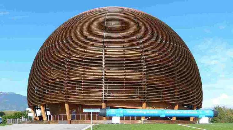
Today, 60 years ago, the visionary convention establishing the European Organization for Nuclear Research – better known with its French acronym, CERN – entered into force, marking the beginning of an extraordinary scientific adventure that has profoundly changed science, technology, and society, and that is still far from over.
With other pan-European institutions established in the late 1940s and early 1950s — like the Council of Europe and the European Coal and Steel Community — CERN shared the same founding goal: to coordinate the efforts of European countries after the devastating losses and large-scale destruction of World War II. Europe had in particular lost its scientific and intellectual leadership, and many scientists had fled to other countries. Time had come for European researchers to join forces towards creating of a world-leading laboratory for fundamental science.
Sixty years after its foundation, CERN is today the largest scientific laboratory in the world, with more than 2000 staff members and many more temporary visitors and fellows. It hosts the most powerful particle accelerator ever built. It also hosts exhibitions, lectures, shows, meetings, and debates, providing a forum of discussion where science meets industry and society.
What has happened in these six decades of scientific research? As a physicist, I should probably first mention the many ground-breaking discoveries in Particle Physics, such as the discovery of some of the most fundamental building block of matter, like the W and Z bosons in 1983; the measurement of the number of neutrino families at LEP in 1989; and of course the recent discovery of the Higgs boson in 2012, which prompted the Nobel Prize in Physics to Peter Higgs and Francois Englert in 2013.
But looking back at the glorious history of this laboratory, much more comes to mind: the development of technologies that found medical applications such as PET scans; computer science applications such as globally distributed computing, that finds application in many fields ranging from genetic mapping to economic modeling; and the World Wide Web, that was developed at CERN as a network to connect universities and research laboratories.
“CERN Control Center (2)” by Martin Dougiamas – Flickr: CERN control center. Licensed under CC BY 2.0 via Wikimedia Commons.
If you’ve ever asked yourself what such a laboratory may look like, especially if you plan to visit it in the future and expect to see building with a distinctive sleek, high-tech look, let me warn you that the first impression may be slightly disappointing. When I first visited CERN, I couldn’t help noticing the old buildings, dusty corridors, and the overall rather grimy look of the section hosting the theory institute. But it was when an elevator brought me down to visit the accelerator that I realized what was actually happening there, as I witnessed the colossal size of the detectors, and the incredible degree of sophistication of the technology used. ATLAS, for instance, is a 25 meters high, 25 meters wide and 45 meters long detector, and it weighs about 7,000 tons!
The 27-km long Large Hadron Collider is currently shut down for planned upgrades. When new beams of protons will be circulated in it at the end of 2014, it will be at almost twice the energy reached in the previous run. There will be about 2800 bunches of protons in its orbit, each containing several hundred billion protons, separated by – as in a car race, the distance between bunches can be expressed in units of time – 250 billionths of a second. The energy of each proton will be compared to that of a flying mosquito, but concentrated in a single elementary particle. And the energy of an entire bunch of protons will be comparable to that of a medium-sized car launched at highway speed.
Why these high energies? Einstein’s E=mc2 tells us that energy can be converted to mass, so by colliding two protons with very high energy, we can in principle produce very heavy particles, possibly new particles that we have never before observed. You may wonder why we would expect that such new particles exist. After all we have already successfully created Higgs bosons through very high-energy collisions, what can we expect to find beyond that? Well, that’s where the story becomes exciting.
Some of the best motivated theories currently under scrutiny in the scientific community – such as Supersymmetry – predict that not only should new particles exist, but they could explain one of the greatest mysteries in Cosmology: the presence of large amounts of unseen matter in the Universe, which seem to dominate the dynamics of all structures in the Universe, including our own Milky Way galaxy — Dark Matter.
Identifying in our accelerators the substance that permeates the Universe and shapes its structure would represent an important step forward in our quest to understand the Cosmos, and our place in it. CERN, 60 years and still going strong, is rising up to challenge.
Headline image credit: An example of simulated data modeled for the CMS particle detector on the Large Hadron Collider (LHC) at CERN. Image by Lucas Taylor, CERN. CC BY-SA 3.0 via Wikimedia Commons.
2014 marks not just the centenary of the start of World War I, and the 75th anniversary of World War II, but on 29 September it is 60 years since the establishment of CERN, the European Centre for Nuclear Research or, in its modern form, Particle Physics. Less than a decade after European nations had been fighting one another in a terrible war, 12 of those nations had united in science. Today, CERN is a world laboratory, famed for having been the home of the world wide web, brainchild of then CERN scientist Tim Berners-Lee; of several Nobel Prizes for physics, although not (yet) for Peace; and most recently, for the discovery of the Higgs Boson. The origin of CERN, and its political significance, are perhaps no less remarkable than its justly celebrated status as the greatest laboratory of scientific endeavour in history.
Its life has spanned a remarkable period in scientific culture. The paradigm shifts in our understanding of the fundamental particles and the forces that control the cosmos, which have occurred since 1950, are in no small measure thanks to CERN.
In 1954, the hoped for simplicity in matter, where the electron and neutrino partner a neutron and proton, had been lost. Novel relatives of the proton were proliferating. Then, exactly 50 years ago, the theoretical concept of the quark was born, which explains the multitude as bound states of groups of quarks. By 1970 the existence of this new layer of reality had been confirmed, by experiments at Stanford, California, and at CERN.
During the 1970s our understanding of quarks and the strong force developed. On the one hand this was thanks to theory, but also due to experiments at CERN’s Intersecting Storage Rings: the ISR. Head on collisions between counter-rotating beams of protons produced sprays of particles, which instead of flying in all directions, tended to emerge in sharp jets. The properties of these jets confirmed the predictions of quantum chromodynamics – QCD – the theory that the strong force arises from the interactions among the fundamental quarks and gluons.
CERN had begun in 1954 with a proton synchrotron, a circular accelerator with a circumference of about 600 metres, which was vast at the time, although trifling by modern standards. This was superseded by a super-proton synchrotron, or SPS, some 7 kilometres in circumference. This fired beams of protons and other particles at static targets, its precision measurements building confidence in the QCD theory and also in the theory of the weak force – QFD, quantum flavourdynamics.
The Globe of Science and Innovation. CC0 via Pixabay
QFD brought the electromagnetic and weak forces into a single framework. This first step towards a possible unification of all forces implied the existence of W and Z bosons, analogues of the photon. Unlike the massless photon, however, the W and Z were predicted to be very massive, some 80 to 90 times more than a proton or neutron, and hence beyond reach of experiments at that time. This changed when the SPS was converted into a collider of protons and anti-protons. By 1984 experiments at the novel accelerator had discovered the W and Z bosons, in line with what QFD predicted. This led to Nobel Prizes for Carlo Rubbia and Simon van der Meer, in 1984.
The confirmation of QCD and QFD led to a marked change in particle physics. Where hitherto it had sought the basic templates of matter, from the 1980s it turned increasingly to understanding how matter emerged from the Big Bang. For CERN’s very high-energy experiments replicate conditions that were prevalent in the hot early universe, and theory implies that the behaviour of the forces and particles in such circumstances is less complex than at the relatively cool conditions of daily experience. Thus began a period of high-energy particle physics as experimental cosmology.
This raced ahead during the 1990s with LEP – the Large Electron Positron collider, a 27 kilometre ring of magnets underground, which looped from CERN towards Lake Geneva, beneath the airport and back to CERN, via the foothills of the Jura Mountains. Initially designed to produce tens of millions of Z bosons, in order to test QFD and QCD to high precision, by 2000 its performance was able to produce pairs of W bosons. The precision was such that small deviations were found between these measurements and what theory implied for the properties of these particles.
The explanation involved two particles, whose subsequent discoveries have closed a chapter in physics. These are the top quark, and the Higgs Boson.
As gaps in Mendeleev’s periodic table of the elements in the 19th century had identified new elements, so at the end of the 20th century a gap in the emerging pattern of particles was discerned. To complete the menu required a top quark.
The precision measurements at LEP could be explained if the top quark exists, too massive for LEP to produce directly, but nonetheless able to disturb the measurements of other quantities at LEP courtesy of quantum theory. Theory and data would agree if the top quark mass were nearly two hundred times that of a proton. The top quark was discovered at Fermilab in the USA in 1995, its mass as required by the LEP data from CERN.
As the 21st century dawned, all the pieces of the “Standard Model” of particles and forces were in place, but one. The theories worked well, but we had no explanation of why the various particles have their menu of masses, or even why they have mass at all. Adding mass into the equations by hand is like a band-aid, capable of allowing computations that agree with data to remarkable precision. However, we can imagine circumstances, where particles collide at energies far beyond those accessible today, where the theories would predict nonsense — infinity as the answer for quantities that are finite, for example. A mathematical solution to this impasse had been discovered fifty years ago, and implied that there is a further massive particle, known as the Higgs Boson, after Peter Higgs who, alone of the independent discoveries of the concept, drew attention to some crucial experimental implications of the boson.
Discovery of the Higgs Boson at CERN in 2012 following the conversion of LEP into the LHC – Large Hadron Collider – is the climax of CERN’s first 60 years. It led to the Nobel Prize for Higgs and Francois Englert, theorists whose ideas initiated the quest. Many wondered whether the Nobel Foundation would break new ground and award the physics prize to a laboratory, CERN, for enabling the experimental discovery, but this did not happen.
CERN has been associated with other Nobel Prizes in Physics, such as to Georges Charpak, for his innovative work developing methods of detecting radiation and particles, which are used not just at CERN but in industry and hospitals. CERN’s reach has been remarkable. From a vision that helped unite Europe, through science, we have seen it breach the Cold War, with collaborations in the 1960s onwards with JINR, the Warsaw Pact’s scientific analogue, and today CERN has become truly a physics laboratory for the world.
René Descartes wrote his third book, Principles of Philosophy, as something of a rival to scholastic textbooks. He prided himself in ‘that those who have not yet learned the philosophy of the schools will learn it more easily from this book than from their teachers, because by the same means they will learn to scorn it, and even the most mediocre teachers will be capable of teaching my philosophy by means of this book alone’ (Descartes to Marin Mersenne, December 1640).
Still, what Descartes produced was inadequate for the task. The topics of scholastic textbooks ranged much more broadly than those of Descartes’ Principles; they usually had four-part arrangements mirroring the structure of the collegiate curriculum, divided as they typically were into logic, ethics, physics, and metaphysics.
But Descartes produced at best only what could be called a general metaphysics and a partial physics.
Knowing what a scholastic course in physics would look like, Descartes understood that he needed to write at least two further parts to his Principles of Philosophy: a fifth part on living things, i.e., animals and plants, and a sixth part on man. And he did not issue what would be called a particular metaphysics.
Portrait of René Descartes by Frans Hans. Public domain viaWikimedia Commons.
Descartes, of course, saw himself as presenting Cartesian metaphysics as well as physics, both the roots and trunk of his tree of philosophy.
But from the point of view of school texts, the metaphysical elements of physics (general metaphysics) that Descartes discussed—such as the principles of bodies: matter, form, and privation; causation; motion: generation and corruption, growth and diminution; place, void, infinity, and time—were usually taught at the beginning of the course on physics.
The scholastic course on metaphysics—particular metaphysics—dealt with other topics, not discussed directly in the Principles, such as: being, existence, and essence; unity, quantity, and individuation; truth and falsity; good and evil.
Such courses usually ended up with questions about knowledge of God, names or attributes of God, God’s will and power, and God’s goodness.
Thus the Principles of Philosophy by itself was not sufficient as a text for the standard course in metaphysics. And Descartes also did not produce texts in ethics or logic for his followers to use or to teach from.
These must have been perceived as glaring deficiencies in the Cartesian program and in the aspiration to replace Aristotelian philosophy in the schools.
So the Cartesians rushed in to fill the voids. One could mention their attempts to complete the physics—Louis de la Forge’s additions to the Treatise on Man, for example—or to produce more conventional-looking metaphysics—such as Johann Clauberg’s later editions of his Ontosophia or Baruch Spinoza’s Metaphysical Thoughts.
Cartesians in the 17th century began to supplement the Principles and to produce the kinds of texts not normally associated with their intellectual movement, that is treatises on ethics and logic, the most prominent of the latter being the Port-Royal Logic (Paris, 1662).
By the end of the 17th century, the Cartesians, having lost many battles, ultimately won the war against the Scholastics.
The attempt to publish a Cartesian textbook that would mirror what was taught in the schools culminated in the famous multi-volume works of Pierre-Sylvain Régis and of Antoine Le Grand.
The Franciscan friar Le Grand initially published a popular version of Descartes’ philosophy in the form of a scholastic textbook, expanding it in the 1670s and 1680s; the work, Institution of Philosophy, was then translated into English together with other texts of Le Grand and published as An Entire Body of Philosophy according to the Principles of the famous Renate Descartes (London, 1694).
On the Continent, Régis issued his General System According to the Principles of Descartes at about the same time (Amsterdam, 1691), having had difficulties receiving permission to publish. Ultimately, Régis’ oddly unsystematic (and very often un-Cartesian) System set the standard for Cartesian textbooks.
By the end of the 17th century, the Cartesians, having lost many battles, ultimately won the war against the Scholastics. The changes in the contents of textbooks from the scholastic Summa at beginning of the 17th century to the Cartesian System at the end can enable one to demonstrate the full range of the attempted Cartesian revolution whose scope was not limited to physics (narrowly conceived) and its epistemology, but included logic, ethics, physics (more broadly conceived), and metaphysics.
Headline image credit: Dispute of Queen Cristina Vasa and René Descartes, by Nils Forsberg (1842-1934) after Pierre-Louis Dumesnil the Younger (1698-1781). Public domain via Wikimedia Commons.
The discovery of the periodic system of the elements and the associated periodic table is generally attributed to the great Russian chemist Dmitri Mendeleev. Many authors have indulged in the game of debating just how much credit should be attributed to Mendeleev and how much to the other discoverers of this unifying theme of modern chemistry.
In fact the discovery of the periodic table represents one of a multitude of multiple discoveries which most accounts of science try to explain away. Multiple discovery is actually the rule rather than the exception and it is one of the many hints that point to the interconnected, almost organic nature of how science really develops. Many, including myself, have explored this theme by considering examples from the history of atomic physics and chemistry.
But today I am writing about a subaltern who discovered the periodic table well before Mendeleev and whose most significant contribution was published on 20 August 1864, or precisely 150 years ago. John Reina Newlands was an English chemist who never held a university position and yet went further than any of his contemporary professional chemists in discovering the all-important repeating pattern among the elements which he described in a number of articles.
Newlands came from Southwark, a suburb of London. After studying at the Royal College of chemistry he became the chief chemist at Royal Agricultural Society of Great Britain. In 1860 when the leading European chemists were attending the Karlsruhe conference to discuss such concepts as atoms, molecules and atomic weights, Newlands was busy volunteering to fight in the Italian revolutionary war under Garibaldi. This is explained by the fact that his mother was Italian descent, which also explains his having the middle name Reina. In any case he survived the fighting and set about thinking about the elements on his return to London to become a sugar chemist.
In 1863 Newlands published a list of elements which he arranged into 11 groups. The elements within each of his groups had analogous properties and displayed weights that differed by eight units or some factor of eight. But no table yet!
Nevertheless he even predicted the existence of a new element, which he believed should have an atomic weight of 163 and should fall between iridium and rhodium. Unfortunately for Newlands neither this element, or a few more he predicted, ever materialized but it does show that the prediction of elements from a system of elements is not something that only Mendeleev invented.
In the first of three articles of 1864 Newlands published his first periodic table, five years before Mendeleev incidentally. This arrangement benefited from the revised atomic weights that had been announced at the Karlsruhe conference he had missed and showed that many elements had weights differing by 16 units. But it only contained 12 elements ranging between lithium as the lightest and chlorine as the heaviest.
Then another article, on 20 August 1864, with a slightly expanded range of elements in which he dropped the use of atomic weights for the elements and replaced them with an ordinal number for each one. Historians and philosophers have amused themselves over the years by debating whether this represents an anticipation of the modern concept of atomic number, but that’s another story.
More importantly Newlands now suggested that he had a system, a repeating and periodic pattern of elements, or a periodic law. Another innovation was Newlands’ willingness to reverse pairs of elements if their atomic weights demanded this change as in the case of tellurium and iodine. Even though tellurium has a higher atomic weight than iodine it must be placed before iodine so that each element falls into the appropriate column according to chemical similarities.
The following year, Newlands had the opportunity to present his findings in a lecture to the London Chemical Society but the result was public ridicule. One member of the audience mockingly asked Newlands whether he had considered arranging the elements alphabetically since this might have produced an even better chemical grouping of the elements. The society declined to publish Newlands’ article although he was able to publish it in another journal.
In 1869 and 1870 two more prominent chemists who held university positions published more elaborate periodic systems. They were the German Julius Lothar Meyer and the Russian Dmitri Mendeleev. They essentially rediscovered what Newlands found and made some improvements. Mendeleev in particular made a point of denying Newlands’ priority claiming that Newlands had not regarded his discovery as representing a scientific law. These two chemists were awarded the lion’s share of the credit and Newlands was reduced to arguing for his priority for several years afterwards. In the end he did gain some recognition when the Davy award, or the equivalent of the Nobel Prize for chemistry at the time, and which had already been jointly awarded to Lothar Meyer and Mendeleev, was finally accorded to Newlands in 1887, twenty three years after his article of August 1864.
But there is a final word to be said on this subject. In 1862, two years before Newlands, a French geologist, Emile Béguyer de Chancourtois had already published a periodic system that he arranged in a three-dimensional fashion on the surface of a metal cylinder. He called this the “telluric screw,” from tellos — Greek for the Earth since he was a geologist and since he was classifying the elements of the earth.
Dmitri Mendeleev believed he was a great scientist and indeed he was. He was not actually recognized as such until his periodic table achieved worldwide diffusion and began to appear in textbooks of general chemistry and in other major publications. When Mendeleev died in February 1907, the periodic table was established well enough to stand on its own and perpetuate his name for upcoming generations of chemists.
The man died, but the myth was born.
Mendeleev as a legendary figure grew with time, aided by his own well-organized promotion of his discovery. Well-versed in foreign languages and with a sort of overwhelming desire to escape his tsar-dominated homeland, he traveled the length and breadth of Europe, attending many conferences in England, Germany, Italy, and central Europe, his only luggage seemingly his periodic table.
Mendeleev had succeeded in creating a new tool that chemists could use as a springboard to new and fascinating discoveries in the fields of theoretical, mineral, and general chemistry. But every coin has two faces, even the periodic table. On the one hand, it lighted the path to the discovery of still missing elements; on the other, it led some unfortunate individuals to fall into the fatal error of announcing the discovery of false or spurious supposed new elements. Even Mendeleev, who considered himself the Newton of the chemical sciences, fell into this trap, announcing the discovery of imaginary elements that presently we know to have been mere self-deception or illusion.
It probably is not well-known that Mendeleev had predicted the existence of a large number of elements, actually more than ten. Their discoveries were sometimes the result of lucky guesses (like the famous cases of gallium, germanium, and scandium), and at other times they were erroneous. Historiography has kindly passed over the latter, forgetting about the long line of imaginary elements that Mendeleev had proposed, among which were two with atomic weights lower than that of hydrogen, newtonium (atomic weight = 0.17) and coronium (Atomic weight = 0.4). He also proposed the existence of six new elements between hydrogen and lithium, whose existence could not but be false.
Mendeleev represented a sort of tormented genius who believed in the universality of his creature and dreaded the possibility that it could be eclipsed by other discoveries. He did not live long enough to see the seed that he had planted become a mighty tree. He fought equally, with fierce indignation, the priority claims of others as well as the advent of new discoveries that appeared to menace his discovery.
In the end, his table was enduring enough to accommodate atomic number, isotopes, radioisotopes, the noble gases, the rare earth elements, the actinides, and the quantum mechanics that endowed it with a theoretical framework, allowing it to appear fresh and modern even after a scientific journey of 145 years.
Image: Nursery of new stars by NASA, Hui Yang University of Illinois. Public domain via Wikimedia Commons.
The past couple of years have seen the celebration of a number of key developments in the history of physics. In 1913 Niels Bohr, perhaps the second most famous physicist of the 20th century after Einstein, published is iconic theory of the atom. Its main ingredient, which has propelled it into the scientific hall of fame, was it’s incorporation of the notion of the quantum of energy. The now commonplace view that electrons are in shells around the nucleus is a direct outcome of the quantization of their energy.
Between 1913 and 1914 the little known English physicist, Henry Moseley, discovered that the use of increasing atomic weights was not the best way to order the elements in the chemist’s periodic table. Instead, Moseley proposed using a whole number sequence to denote a property that he called the atomic number of an element. This change had the effect of removing the few remaining anomalies in the way that the elements are arranged in this icon of science that is found on the walls of lecture halls and laboratories all over the world. In recent years the periodic table has even become a cultural icon to be appropriated by artists, designers and advertisers of every persuasion.
But another scientist who was publishing articles at about the same time as Bohr and Moseley has been almost completely forgotten by all but a few historians of physics. He is the English mathematical physicist John Nicholson, who was in fact the first to suggest that the momentum of electrons in an atom is quantized. Bohr openly acknowledges this point in all his early papers.
Nicholson hypothesized the existence of what he called proto-elements that he believed existed in inter-stellar space and which gave rise to our familiar terrestrial chemical elements. He gave them exotic names like nebulium and coronium and using this idea he was able to explain many unassigned lines in the spectra of the solar corona and the major stellar nebulas such as the famous Crab nebula in the constellation of Orion. He also succeeded in predicting some hitherto unknown lines in each of these astronomical bodies.
The really odd thing is that Nicholson was completely wrong, or at least that’s how his ideas are usually regarded. How it is that supposedly ‘wrong’ theories can produce such advances in science, even if only temporarily?
Science progresses as a unified whole, not stopping to care about which scientist is successful or not, while being only concerned with overall progress. The attribution of priority and scientific awards, from a global perspective, is a kind of charade which is intended to reward scientists for competing with each other. On this view no scientific development can be regarded as being right or wrong. I like to draw an analogy with the evolution of species or organisms. Developments that occur in living organisms can never be said to be right or wrong. Those that are advantageous to the species are perpetuated while those that are not simply die away. So it is with scientific developments. Nicholson’s belief in proto-elements may not have been productive but his notion of quantization in atoms was tremendously useful and the baton was passed on to Bohr and all the quantum physicists who came later.
Instead of viewing the development of science through the actions of individuals and scientific heroes, a more holistic view is better to discern the whole process — including the work of lesser-known intermediate figures, such as Nicholson. The Dutch economist Anton den Broek first made the proposal that elements should be characterized by an ordinal number before Moseley had even begun doing physics. This is not a disputed point since Moseley begins one of his key papers by stating that he began his research in order to verify the van den Broek hypothesis on atomic number.
Another intermediate figure in the history of physics was Edmund Stoner who took a decisive step forward in assigning quantum numbers to each of the electrons in an atom while as a graduate student at Cambridge. In all there are four such quantum numbers which are used to specify precisely how the electrons are arranged first in shells, then sub-shells and finally orbitals in any atom. Stoner was responsible for applying the third quantum number. It was after reading Stoner’s article that the much more famous Wolfgang Pauli was able to suggest a fourth quantum number which later acquired the name of electron spin to describe a further degree of freedom for every electron in an atom.
Eric Scerri is a full-time chemistry lecturer at UCLA. Eric Scerri is a leading philosopher of science specializing in the history and philosophy of the periodic table. He is also the founder and editor in chief of the international journal Foundations of Chemistry and has been a full-time lecturer at UCLA for the past fifteen years where he regularly teaches classes of 350 chemistry students as well as classes in history and philosophy of science. He is the author of A Tale of Seven Elements,The Periodic Table: Its Story and Its Significance, and The Periodic Table: A Very Short Introduction.
Chemistry Giveaway! In time for the 2014 American Chemical Society fall meeting and in honor of the publication of The Oxford Handbook of Food Fermentations, edited by Charles W. Bamforth and Robert E. Ward, Oxford University Press is running a paired giveaway with this new handbook and Charles Bamforth’s other must-read book, the third edition of Beer. The sweepstakes ends on Thursday, August 14th at 5:30 p.m. EST.
Subscribe to the OUPblog via email or RSS.
Subscribe to only physics and chemistry articles on the OUPblog via email or RSS.
Lipids (fats and oils) have historically been thought to elevate weight and blood cholesterol and have therefore been considered to have a negative influence on the body. Foods such as full-fat milk and cheese have been avoided by many consumers for this reason. This attitude has been changing in recent years. Some authors are now claiming that consumption of unnecessary carbohydrates rather than fat is responsible for the epidemics of obesity and type 2 diabetes mellitus (T2DM). Most people who do consume milk, cheese, and yogurt know that the calcium helps with bones and teeth, but studies have shown that consumption of cheese and other dairy products appears to be beneficial in many other ways. Remember that cheese is a concentrated form of milk. Milk is 87% water and when it is processed into cheese, the nutrients are increased by a factor of ten. The positive attributes of milk are even stronger in cheese. Here are some examples involving protein:
Some bioactive peptides in casein (the primary protein in cheese) inhibit angiotensin-converting enzyme, which has been implicated in hypertension. Large studies have shown that dairy intake reduces blood pressure.
Cheese helps prevent tooth decay through a combination of bacterial inhibition and remineralization. Further, Lactoferrin, a minor milk protein found in cheese, has anticancer properties. It appears to keep cancer cells from proliferating.
Vitamins and minerals in cheese may not get enough credit. A meta-analysis of 16 studies showed that consumption of 200 g of cheese and other dairy products per day resulted in a 6% reduction of risk of T2DM, with a significant association between reduction of incidence of T2DM and intake of cheese, yogurt, and low-fat dairy products. Much of this may be due to vitamin K2, which is produced by bacteria in fermented dairy products.
Metabolic syndrome increases the risk for T2DM and heart disease, but research showed that the incidence of this syndrome decreased as dairy food consumption increased, a result that was associated with calcium intake.
There is evidence that lipids in cheese are not unhealthy after all. Recent research has shown no connection between the intake of milk fat and the risk of cardiovascular disease, coronary heart disease, or stroke. A meta-analysis of 76 studies concluded that the evidence does not clearly support guidelines that encourage high consumption of polyunsaturated fatty acids and low consumption of total saturated fats.
Participants in a study who ate cheese and other dairy products at least once per day scored significantly higher in several tests of cognitive function compared with those who rarely or never consumed dairy food. These results appear to be due to a combination of factors.
Seemingly, the opposite of what people believe about cheese turns out to be the truth. Studies involving thousands of people over a period of years revealed that a high intake of dairy fat was associated with a lower risk of developing central obesity and a low dairy fat intake was associated with a higher risk of central obesity. Higher consumption of cheese has been associated with higher HDL (“good cholesterol”) and lower LDL (“bad cholesterol”), total cholesterol, and triglycerides.
All-cause mortality showed a reduction associated with dairy food intake in a meta-analysis of five studies in England and Wales covering 509,000 deaths in 2008. The authors concluded that there was a large mismatch between evidence from long-term studies and perceptions of harm from dairy foods.
Yes, some people are allergic to protein in cheese and others are vegetarians who don’t touch dairy products on principle. Many people can’t digest lactose (milk sugar) very well, but aged cheese contains little of it and lactose-free cheese has been on the market for years. But cheese is quite healthy for most consumers. Moderation in food consumption is always the key: as long as you eat cheese in reasonable amounts, you ought to have no ill effects while reaping the benefits.
Michael Tunick is a research chemist with the Dairy and Functional Foods Research Unit of the U.S. Department of Agriculture’s Agricultural Research Service. He is the author of The Science of Cheese. You can find out more things you never knew about cheese.
Chemistry Book Giveaway! In time for the 2014 American Chemical Society fall meeting and in honor of the publication of The Oxford Handbook of Food Fermentations, edited by Charles W. Bamforth and Robert E. Ward, Oxford University Press is running a paired giveaway with this new handbook and Charles Bamforth’s other must-read book, the third edition of Beer. The sweepstakes ends on Thursday, August 14th at 5:30 p.m. EST.
Subscribe to the OUPblog via email or RSS.
Subscribe to only physics and chemistry articles on the OUPblog via email or RSS.
Image credit: Hand milking a cow, by the State Library of Australia. CC-BY-2.0 via Wikimedia Commons.


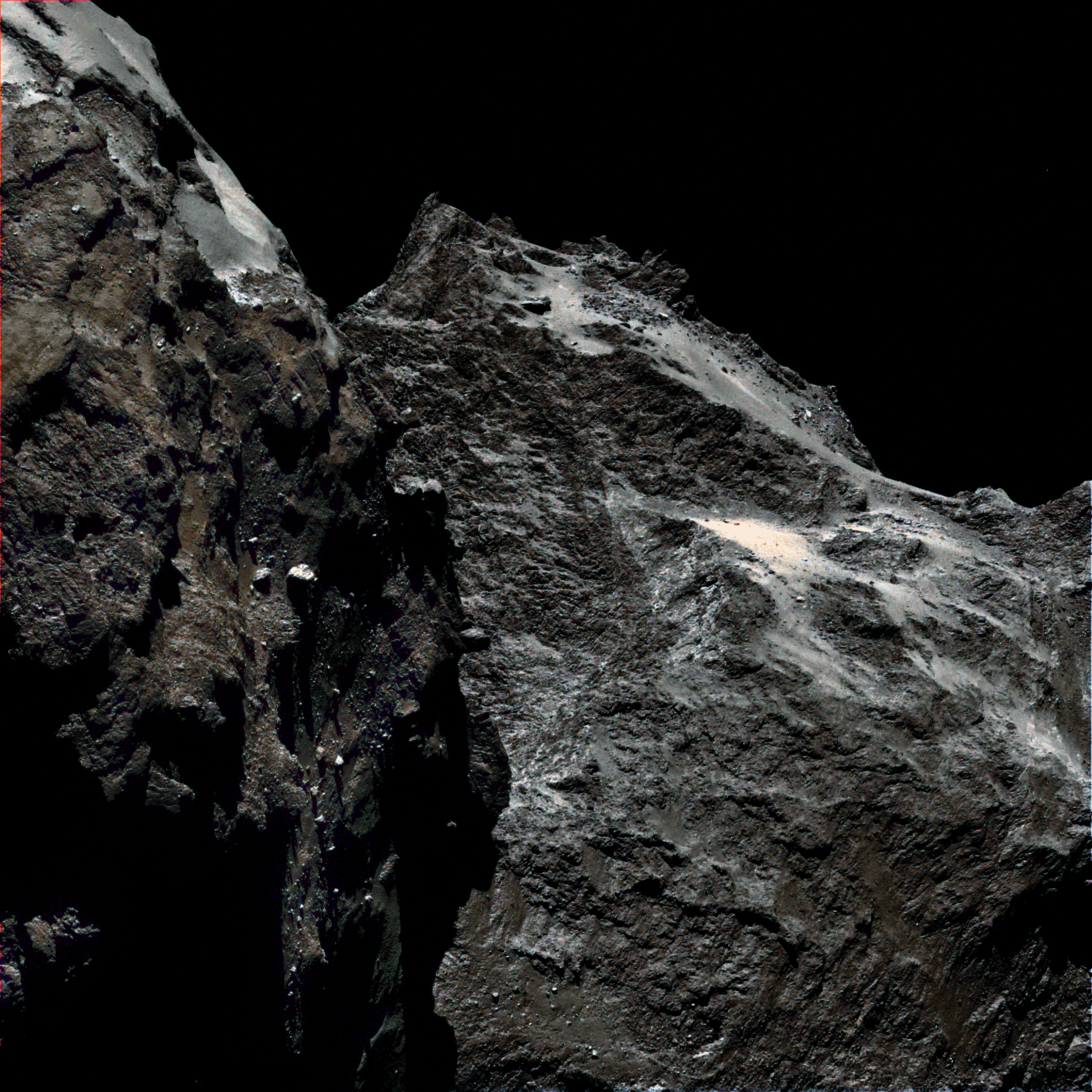
.jpg#mediaviewer/File:CERN_Control_Center_(2).jpg)